Least Squares Regression - Examples

The idea

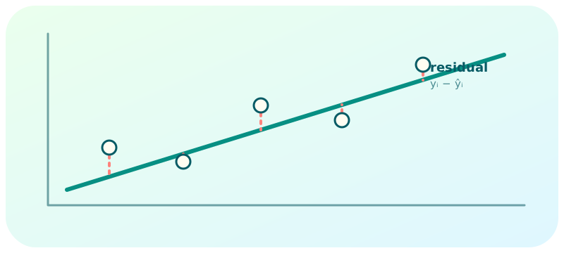
Given observations $(x_i,y_i)$, simple linear regression looks for a line $y=mx+b$. A residual is the vertical difference $y_i-(mx_i+b)$ between an observation and the prediction.

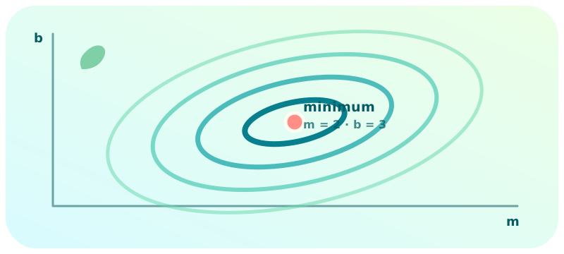
Least squares chooses $m$ and $b$ by minimizing the sum of squared residuals:

$E(m,b)=\sum_{i=1}^{n}\left(y_i-(mx_i+b)\right)^2.$

Squaring prevents positive and negative residuals from cancelling and penalizes large errors. For nonconstant input values, this objective is convex and has a unique minimum.

One explanatory variable

For a simple regression, differentiating $E(m,b)$ with respect to $m$ and $b$ gives

$\hat m=\frac{\sum_{i=1}^n(x_i-\bar x)(y_i-\bar y)}{\sum_{i=1}^n(x_i-\bar x)^2},\qquad \hat b=\bar y-\hat m\bar x.$

The denominator is nonzero when the observed $x_i$ are not all identical.

Several explanatory variables

For $n$ observations and $p$ explanatory variables, collect the observations in a design matrix $X\in\mathbb R^{n\times(p+1)}$. Its first column contains ones for the intercept; each remaining column contains one feature. Put the unknown coefficients in $\beta\in\mathbb R^{p+1}$ and the observed targets in $y\in\mathbb R^n$:

$y=X\beta+\varepsilon.$

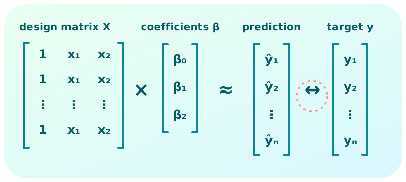
The least-squares estimator is

$\hat\beta=\operatorname*{arg\,min}_{\beta}\|X\beta-y\|_2^2.$

The gradient is

$\nabla_{\beta}\|X\beta-y\|_2^2=2X^T(X\beta-y).$

At a minimum it vanishes, which gives the normal equations

$X^TX\hat\beta=X^Ty.$

If $X$ has full column rank, $X^TX$ is invertible and

$\hat\beta=(X^TX)^{-1}X^Ty.$

Without full column rank, minimizers may not be unique. The minimum-norm solution is $\hat\beta=X^+y$, where $X^+$ is the Moore–Penrose pseudoinverse. Numerical software normally uses a QR or singular-value decomposition instead of explicitly computing $(X^TX)^{-1}$.

Python example

The following example generates noisy observations around $y=2x+3$ and solves the regression with numpy.linalg.lstsq:

import numpy as np

rng = np.random.default_rng(42)
x = np.linspace(0, 10, 100)
y = 2 * x + 3 + rng.normal(0, 1, len(x))

X = np.column_stack((x, np.ones(len(x))))
coefficients, residuals, rank, singular_values = np.linalg.lstsq(
    X, y, rcond=None
)

slope, intercept = coefficients
predictions = X @ coefficients
print(slope, intercept)

The same construction works with more features: add one column to $X$ for each feature. The fitted object then becomes a hyperplane in the feature space; it is not obtained by intersecting separate hyperplanes.